This post is a tutorial on solving the Kaggle Titanic Competition using Deep Neural Network with the TensorFlow API Keras. Kaggle is a competition site which provides problems to solve or questions to ask while providing the datasets for training your data science model and testing the model results against a test dataset. The Titanic competition is probably the first competition you will come across on Kaggle. The goal of the competition is to predict the possibility of survival of the passengers onboard, a typical classification problem.
This tutorial follows a typical workflow of machine learning project.
- Define the problem
- Acquire the data
- Prepare the data
- Define the model
- Train and fine-tune the model
- Test and deploy the model
The accompanying notebook of this tutorial is available here.
Define the problem
The question or problem definition for Titanic Survival competition is described here at Kaggle.
Knowing from a training set of samples listing passengers who survived or did not survive the Titanic disaster, can our model determine based on a given test dataset not containing the survival information, if these passengers in the test dataset survived or not.
Kaggle already provides some early understanding about the domain of this problem, see the Kaggle competition description page here. Here are the highlights to note.
- On April 15, 1912, during her maiden voyage, the Titanic sank after colliding with an iceberg, killing 1502 out of 2224 passengers and crew. Translated 32% survival rate.
- One of the reasons that the shipwreck led to such loss of life was that there were not enough lifeboats for the passengers and crew.
- Although there was some element of luck involved in surviving the sinking, some groups of people were more likely to survive than others, such as women, children, and the upper-class.
Before going forward, we need to import some necessary modules.
1
2
3
4
5
6
7
8
9
10
11
12
13
14
15
16
17
18
| # data analysis
import numpy as np
import pandas as pd
# visualization
import matplotlib.pyplot as plt
import seaborn as sns
# machine learning
import sklearn
from sklearn.model_selection import train_test_split
import tensorflow as tf
from tensorflow.python.framework import ops
# utils
import warnings
warnings.filterwarnings('ignore')
%matplotlib inline
|
Acquire the data
The Python Pandas packages are used to acquire the data. The data consists of two groups: a training set (train.csv) and test set (test.csv).
The training set should be used to build the machine learning models. For the training set, the outcome (also known as the “ground truth”) for each passenger is provided.
The test set should be used to see how well your model performs on unseen data. For the test set, the ground truth for each passenger is not provided. The machine learning models will be used to predict the surival of each passenger.
1
2
| train_data = pd.read_csv('./Dataset/train.csv')
test_data = pd.read_csv('./Dataset/test.csv')
|
| PassengerId | Survived | Pclass | Name | Sex | Age | SibSp | Parch | Ticket | Fare | Cabin | Embarked |
|---|
| 0 | 1 | 0 | 3 | Braund, Mr. Owen Harris | male | 22.0 | 1 | 0 | A/5 21171 | 7.2500 | NaN | S |
|---|
| 1 | 2 | 1 | 1 | Cumings, Mrs. John Bradley (Florence Briggs Th... | female | 38.0 | 1 | 0 | PC 17599 | 71.2833 | C85 | C |
|---|
| 2 | 3 | 1 | 3 | Heikkinen, Miss. Laina | female | 26.0 | 0 | 0 | STON/O2. 3101282 | 7.9250 | NaN | S |
|---|
| 3 | 4 | 1 | 1 | Futrelle, Mrs. Jacques Heath (Lily May Peel) | female | 35.0 | 1 | 0 | 113803 | 53.1000 | C123 | S |
|---|
| 4 | 5 | 0 | 3 | Allen, Mr. William Henry | male | 35.0 | 0 | 0 | 373450 | 8.0500 | NaN | S |
|---|
| PassengerId | Pclass | Name | Sex | Age | SibSp | Parch | Ticket | Fare | Cabin | Embarked |
|---|
| 0 | 892 | 3 | Kelly, Mr. James | male | 34.5 | 0 | 0 | 330911 | 7.8292 | NaN | Q |
|---|
| 1 | 893 | 3 | Wilkes, Mrs. James (Ellen Needs) | female | 47.0 | 1 | 0 | 363272 | 7.0000 | NaN | S |
|---|
| 2 | 894 | 2 | Myles, Mr. Thomas Francis | male | 62.0 | 0 | 0 | 240276 | 9.6875 | NaN | Q |
|---|
| 3 | 895 | 3 | Wirz, Mr. Albert | male | 27.0 | 0 | 0 | 315154 | 8.6625 | NaN | S |
|---|
| 4 | 896 | 3 | Hirvonen, Mrs. Alexander (Helga E Lindqvist) | female | 22.0 | 1 | 1 | 3101298 | 12.2875 | NaN | S |
|---|
Prepare the data
This step aims to prepare the data for use in machine learning training. It involves cleaning up the data, understanding its structure and attributes, studying possible correlations between attributes, and visualizing the data to extract human-level insight on its properties, distribution, range, and overall usefulness [3].
Data Overview
1
2
3
| train_data.info()
print("-" * 40)
test_data.info()
|
1
2
3
4
5
6
7
8
9
10
11
12
13
14
15
16
17
18
19
20
21
22
23
24
25
26
27
28
29
30
31
32
33
34
35
36
37
38
| <class 'pandas.core.frame.DataFrame'>
RangeIndex: 891 entries, 0 to 890
Data columns (total 12 columns):
# Column Non-Null Count Dtype
--- ------ -------------- -----
0 PassengerId 891 non-null int64
1 Survived 891 non-null int64
2 Pclass 891 non-null int64
3 Name 891 non-null object
4 Sex 891 non-null object
5 Age 714 non-null float64
6 SibSp 891 non-null int64
7 Parch 891 non-null int64
8 Ticket 891 non-null object
9 Fare 891 non-null float64
10 Cabin 204 non-null object
11 Embarked 889 non-null object
dtypes: float64(2), int64(5), object(5)
memory usage: 83.7+ KB
----------------------------------------
<class 'pandas.core.frame.DataFrame'>
RangeIndex: 418 entries, 0 to 417
Data columns (total 11 columns):
# Column Non-Null Count Dtype
--- ------ -------------- -----
0 PassengerId 418 non-null int64
1 Pclass 418 non-null int64
2 Name 418 non-null object
3 Sex 418 non-null object
4 Age 332 non-null float64
5 SibSp 418 non-null int64
6 Parch 418 non-null int64
7 Ticket 418 non-null object
8 Fare 417 non-null float64
9 Cabin 91 non-null object
10 Embarked 418 non-null object
dtypes: float64(2), int64(4), object(5)
memory usage: 36.0+ KB
|
Observations
- The data contains 11 features. The details of these features are described on the Kaggle data pape here.
- Categorical: Sex and Embarked,
- Orinial: Pclass,
- Numerical: Age and Fare (continous), SibSp and Parch (discret),
- Mixed: Cabin (alphanumeric).
- There are missing values in Age, Cabin, Embarked and Fare.
Primary data analysis and visualization
1
2
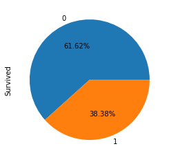
| # Overall Surival Rate
train_data['Survived'].value_counts().plot.pie(autopct = '%1.2f%%');
|
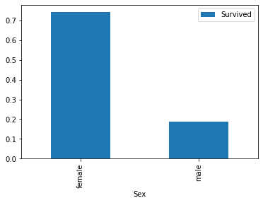
Sex
1
2
| # Sex
train_data[['Sex','Survived']].groupby(['Sex']).mean().plot.bar();
|
Observation: Female passengers had higher survival chance.
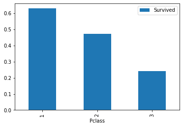
Class
1
2
| # Class
train_data[['Pclass', 'Survived']].groupby('Pclass').mean().plot.bar();
|
Observation: Surival rate Class 1 > Class 2 > Class 3
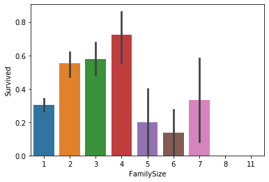
Family size
1
2
3
4
5
| # Family Size
train_data['FamilySize'] = train_data['Parch'] + train_data['SibSp'] + 1
test_data['FamilySize'] = test_data['Parch'] + test_data['SibSp'] + 1
sns.barplot(data=train_data, x='FamilySize', y='Survived');
|
Observation: Passengers with small family size (2-4) were more likely to survive.
Therefore, the passengers are grouped into 3 groups according the size of family: singleton, SmallFamily (family size 2-4) and LargeFamily (family size larger than 4).
1
2
3
4
5
6
7
8
| # Feature engineering
train_data['Singleton'] = train_data['FamilySize'].map(lambda s: 1 if s == 1 else 0)
train_data['SmallFamily'] = train_data['FamilySize'].map(lambda s: 1 if 2<= s <= 4 else 0)
train_data['LargeFamily'] = train_data['FamilySize'].map(lambda s: 1 if s>=5 else 0)
test_data['Singleton'] = test_data['FamilySize'].map(lambda s: 1 if s == 1 else 0)
test_data['SmallFamily'] = test_data['FamilySize'].map(lambda s: 1 if 2<= s <= 4 else 0)
test_data['LargeFamily'] = test_data['FamilySize'].map(lambda s: 1 if s>=5 else 0)
|
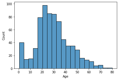
Age
1
2
3
| # Age & Survival Rate
age_data = train_data[train_data['Age'].notna()][['Age', 'Survived']]
sns.histplot(age_data['Age']);
|
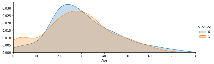
1
2
3
4
| ageFacet=sns.FacetGrid(train_data,hue='Survived',aspect=3);
ageFacet.map(sns.kdeplot,'Age',shade=True);
ageFacet.set(xlim=(0,train_data['Age'].max()));
ageFacet.add_legend();
|
Observation: Passengers aged under 10 were more likely to survive.
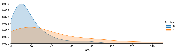
Fare
1
2
3
4
5
| # Fare & Survival Rate
fareFacet=sns.FacetGrid(train_data,hue='Survived',aspect=3);
fareFacet.map(sns.kdeplot,'Fare',shade=True);
fareFacet.set(xlim=(0,150));
fareFacet.add_legend();
|
Observation: Low survival rate for fare < 20.
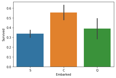
Embarked port
1
2
| # Embarked & Survival Rate
sns.barplot(data=train_data,x='Embarked',y='Survived');
|
Observations: Passengers embarked from port C were more likely to survive.
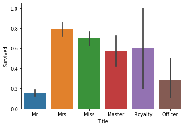
Name (Title)
The titles of the passengers can be extracted from their names. Passengers from different social classes may have different survival chance.
1
2
3
4
| # Extract titles
train_data['Title'] = train_data.Name.str.extract(' ([A-Za-z]+)\.', expand=False)
test_data['Title'] = test_data.Name.str.extract(' ([A-Za-z]+)\.', expand=False)
train_data['Title'].value_counts()
|
1
2
3
4
5
6
7
8
9
10
11
12
13
14
15
16
17
18
| Mr 517
Miss 182
Mrs 125
Master 40
Dr 7
Rev 6
Mlle 2
Major 2
Col 2
Ms 1
Don 1
Lady 1
Mme 1
Sir 1
Countess 1
Capt 1
Jonkheer 1
Name: Title, dtype: int64
|
1
2
3
4
5
6
7
8
9
10
11
12
13
14
15
16
17
18
19
20
21
22
23
24
| # Group the passengers into 6 groups by their titles.
Title_Dictionary = {
"Capt": "Officer",
"Col": "Officer",
"Major": "Officer",
"Jonkheer": "Royalty",
"Don": "Royalty",
"Sir" : "Royalty",
"Dr": "Officer",
"Rev": "Officer",
"Countess": "Royalty",
"Dona": "Royalty",
"Mme": "Mrs",
"Mlle": "Miss",
"Ms": "Mrs",
"Mr" : "Mr",
"Mrs" : "Mrs",
"Miss" : "Miss",
"Master" : "Master",
"Lady" : "Royalty"
}
train_data['Title']=train_data['Title'].map(Title_Dictionary)
test_data['Title']=test_data['Title'].map(Title_Dictionary)
train_data['Title'].value_counts()
|
1
2
3
4
5
6
7
| Mr 517
Miss 184
Mrs 127
Master 40
Officer 18
Royalty 5
Name: Title, dtype: int64
|
1
| sns.barplot(data=train_data, x='Title', y='Survived');
|
Observation: Passengers with “Mr” and “Officer” titles had low survival chance.
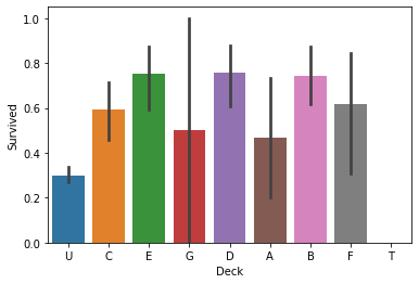
Cabin
The Cabin information can tell which decks the passengers were resided, which may influence the survival rate. The Cabin variables have many missing values. THe missing values will be replaced by “Unknown”.
1
2
| train_data['Cabin'] = train_data['Cabin'].fillna('Unknown')
test_data['Cabin'] = test_data['Cabin'].fillna('Unknown')
|
1
2
3
4
| # Cabin
train_data['Deck']=train_data['Cabin'].map(lambda x:x[0])
test_data['Deck']=test_data['Cabin'].map(lambda x:x[0])
sns.barplot(data=train_data, x='Deck', y='Survived');
|
Observation: Passengers in Deck B, D, E were more likely to survive.
Data pre-processing
Combine all data
1
| full_data = pd.concat([train_data, test_data], axis=0)
|
Fill the missing values
Embarked
1
2
| # Embarked
full_data[full_data['Embarked'].isnull()]
|
| PassengerId | Survived | Pclass | Name | Sex | Age | SibSp | Parch | Ticket | Fare | Cabin | Embarked | FamilySize | Singleton | SmallFamily | LargeFamily | Title | Deck |
|---|
| 61 | 62 | 1.0 | 1 | Icard, Miss. Amelie | female | 38.0 | 0 | 0 | 113572 | 80.0 | B28 | NaN | 1 | 1 | 0 | 0 | Miss | B |
|---|
| 829 | 830 | 1.0 | 1 | Stone, Mrs. George Nelson (Martha Evelyn) | female | 62.0 | 0 | 0 | 113572 | 80.0 | B28 | NaN | 1 | 1 | 0 | 0 | Mrs | B |
|---|
1
| full_data['Embarked'].value_counts()
|
1
2
3
4
| S 914
C 270
Q 123
Name: Embarked, dtype: int64
|
Fill the missing value of the Embarked feature with the most frequent value.
1
| full_data['Embarked'] = full_data['Embarked'].fillna('S')
|
Fare
1
2
| # Fare
full_data[full_data['Fare'].isnull()]
|
| PassengerId | Survived | Pclass | Name | Sex | Age | SibSp | Parch | Ticket | Fare | Cabin | Embarked | FamilySize | Singleton | SmallFamily | LargeFamily | Title | Deck |
|---|
| 152 | 1044 | NaN | 3 | Storey, Mr. Thomas | male | 60.5 | 0 | 0 | 3701 | NaN | Unknown | S | 1 | 1 | 0 | 0 | Mr | U |
|---|
Fill the missing value of the Fare feature with the mean value.
1
| full_data['Fare']=full_data['Fare'].fillna(full_data[(full_data['Pclass']==3)&(full_data['Embarked']=='S')&(full_data['Cabin']=='Unknown')]['Fare'].mean())
|
Age
The Random Forest algorithm is used to fill the missing of the Age feature.
1
2
3
| AgePre = full_data[['Age','Pclass','Title','FamilySize','Sex']]
AgePre = pd.get_dummies(AgePre)
AgePre.head()
|
| Age | Pclass | FamilySize | Title_Master | Title_Miss | Title_Mr | Title_Mrs | Title_Officer | Title_Royalty | Sex_female | Sex_male |
|---|
| 0 | 22.0 | 3 | 2 | 0 | 0 | 1 | 0 | 0 | 0 | 0 | 1 |
|---|
| 1 | 38.0 | 1 | 2 | 0 | 0 | 0 | 1 | 0 | 0 | 1 | 0 |
|---|
| 2 | 26.0 | 3 | 1 | 0 | 1 | 0 | 0 | 0 | 0 | 1 | 0 |
|---|
| 3 | 35.0 | 1 | 2 | 0 | 0 | 0 | 1 | 0 | 0 | 1 | 0 |
|---|
| 4 | 35.0 | 3 | 1 | 0 | 0 | 1 | 0 | 0 | 0 | 0 | 1 |
|---|
1
2
3
4
5
6
7
8
9
10
11
12
13
14
15
16
| # Split the dateset
AgeKnown=AgePre[AgePre['Age'].notnull()]
AgeUnKnown=AgePre[AgePre['Age'].isnull()]
AgeKnown_X=AgeKnown.drop(['Age'],axis=1)
AgeKnown_y=AgeKnown['Age']
AgeUnKnown_X=AgeUnKnown.drop(['Age'],axis=1)
# Setup the random forest model
from sklearn.ensemble import RandomForestRegressor
rfr=RandomForestRegressor(random_state=None,n_estimators=500,n_jobs=-1)
rfr.fit(AgeKnown_X,AgeKnown_y)
# Model evaluation
rfr.score(AgeKnown_X,AgeKnown_y)
|
1
2
3
4
5
6
7
| # Predict age
AgeUnKnown_y=rfr.predict(AgeUnKnown_X)
# Fill the mssing value
full_data.loc[full_data['Age'].isnull(),['Age']]=AgeUnKnown_y
# Create featuer IsChild (less than 10 years old)
full_data['IsChild'] = full_data['Age'].map(lambda s: 1 if s <= 10 else 0)
full_data.info() # no missing values now (except Survived)
|
1
2
3
4
5
6
7
8
9
10
11
12
13
14
15
16
17
18
19
20
21
22
23
24
25
26
| <class 'pandas.core.frame.DataFrame'>
Int64Index: 1309 entries, 0 to 417
Data columns (total 19 columns):
# Column Non-Null Count Dtype
--- ------ -------------- -----
0 PassengerId 1309 non-null int64
1 Survived 891 non-null float64
2 Pclass 1309 non-null int64
3 Name 1309 non-null object
4 Sex 1309 non-null object
5 Age 1309 non-null float64
6 SibSp 1309 non-null int64
7 Parch 1309 non-null int64
8 Ticket 1309 non-null object
9 Fare 1309 non-null float64
10 Cabin 1309 non-null object
11 Embarked 1309 non-null object
12 FamilySize 1309 non-null int64
13 Singleton 1309 non-null int64
14 SmallFamily 1309 non-null int64
15 LargeFamily 1309 non-null int64
16 Title 1309 non-null object
17 Deck 1309 non-null object
18 IsChild 1309 non-null int64
dtypes: float64(3), int64(9), object(7)
memory usage: 204.5+ KB
|
| PassengerId | Survived | Pclass | Name | Sex | Age | SibSp | Parch | Ticket | Fare | Cabin | Embarked | FamilySize | Singleton | SmallFamily | LargeFamily | Title | Deck | IsChild |
|---|
| 0 | 1 | 0.0 | 3 | Braund, Mr. Owen Harris | male | 22.0 | 1 | 0 | A/5 21171 | 7.2500 | Unknown | S | 2 | 0 | 1 | 0 | Mr | U | 0 |
|---|
| 1 | 2 | 1.0 | 1 | Cumings, Mrs. John Bradley (Florence Briggs Th... | female | 38.0 | 1 | 0 | PC 17599 | 71.2833 | C85 | C | 2 | 0 | 1 | 0 | Mrs | C | 0 |
|---|
| 2 | 3 | 1.0 | 3 | Heikkinen, Miss. Laina | female | 26.0 | 0 | 0 | STON/O2. 3101282 | 7.9250 | Unknown | S | 1 | 1 | 0 | 0 | Miss | U | 0 |
|---|
| 3 | 4 | 1.0 | 1 | Futrelle, Mrs. Jacques Heath (Lily May Peel) | female | 35.0 | 1 | 0 | 113803 | 53.1000 | C123 | S | 2 | 0 | 1 | 0 | Mrs | C | 0 |
|---|
| 4 | 5 | 0.0 | 3 | Allen, Mr. William Henry | male | 35.0 | 0 | 0 | 373450 | 8.0500 | Unknown | S | 1 | 1 | 0 | 0 | Mr | U | 0 |
|---|
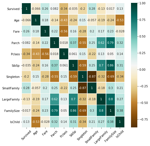
Select the features
1
2
3
4
5
6
| # Remove the less revelant features
fullSel=full_data.drop(['Cabin','Name','Ticket','PassengerId'],axis=1)
# Check the correlations of the features
corrDf=pd.DataFrame()
corrDf=fullSel.corr()
corrDf['Survived'].sort_values(ascending=True)
|
1
2
3
4
5
6
7
8
9
10
11
12
| Pclass -0.338481
Singleton -0.203367
LargeFamily -0.125147
Age -0.065783
SibSp -0.035322
FamilySize 0.016639
Parch 0.081629
IsChild 0.125678
Fare 0.257307
SmallFamily 0.279855
Survived 1.000000
Name: Survived, dtype: float64
|
1
2
3
4
5
6
| # Heatmap
plt.figure(figsize=(8,8));
sns.heatmap(fullSel[['Survived','Age','Embarked','Fare','Parch','Pclass',
'Sex','SibSp','Title','Singleton','SmallFamily','LargeFamily','FamilySize','IsChild','Deck']].corr(),cmap='BrBG',annot=True,
linewidths=.5);
plt.xticks(rotation=45);
|
1
| fullSel=fullSel.drop(['SibSp','Parch','FamilySize','Age'],axis=1)
|
One-hot encoding
1
2
3
| # One-hot encoding
fullSel=pd.get_dummies(fullSel)
PclassDf=pd.get_dummies(full_data['Pclass'],prefix='Pclass')
|
| Pclass_1 | Pclass_2 | Pclass_3 |
|---|
| 0 | 0 | 0 | 1 |
|---|
| 1 | 1 | 0 | 0 |
|---|
| 2 | 0 | 0 | 1 |
|---|
| 3 | 1 | 0 | 0 |
|---|
| 4 | 0 | 0 | 1 |
|---|
1
| fullSel = pd.concat([fullSel, PclassDf], axis=1)
|
1
| fullSel.drop('Pclass', axis=1, inplace=True)
|
| Survived | Fare | Singleton | SmallFamily | LargeFamily | IsChild | Sex_female | Sex_male | Embarked_C | Embarked_Q | ... | Deck_C | Deck_D | Deck_E | Deck_F | Deck_G | Deck_T | Deck_U | Pclass_1 | Pclass_2 | Pclass_3 |
|---|
| 0 | 0.0 | 7.2500 | 0 | 1 | 0 | 0 | 0 | 1 | 0 | 0 | ... | 0 | 0 | 0 | 0 | 0 | 0 | 1 | 0 | 0 | 1 |
|---|
| 1 | 1.0 | 71.2833 | 0 | 1 | 0 | 0 | 1 | 0 | 1 | 0 | ... | 1 | 0 | 0 | 0 | 0 | 0 | 0 | 1 | 0 | 0 |
|---|
| 2 | 1.0 | 7.9250 | 1 | 0 | 0 | 0 | 1 | 0 | 0 | 0 | ... | 0 | 0 | 0 | 0 | 0 | 0 | 1 | 0 | 0 | 1 |
|---|
| 3 | 1.0 | 53.1000 | 0 | 1 | 0 | 0 | 1 | 0 | 0 | 0 | ... | 1 | 0 | 0 | 0 | 0 | 0 | 0 | 1 | 0 | 0 |
|---|
| 4 | 0.0 | 8.0500 | 1 | 0 | 0 | 0 | 0 | 1 | 0 | 0 | ... | 0 | 0 | 0 | 0 | 0 | 0 | 1 | 0 | 0 | 1 |
|---|
5 rows × 29 columns
Normalization
1
| fullSel[fullSel.columns] = fullSel[fullSel.columns].apply(lambda x: x/x.max(), axis=0)
|
| Survived | Fare | Singleton | SmallFamily | LargeFamily | IsChild | Sex_female | Sex_male | Embarked_C | Embarked_Q | ... | Deck_C | Deck_D | Deck_E | Deck_F | Deck_G | Deck_T | Deck_U | Pclass_1 | Pclass_2 | Pclass_3 |
|---|
| 0 | 0.0 | 0.014151 | 0.0 | 1.0 | 0.0 | 0.0 | 0.0 | 1.0 | 0.0 | 0.0 | ... | 0.0 | 0.0 | 0.0 | 0.0 | 0.0 | 0.0 | 1.0 | 0.0 | 0.0 | 1.0 |
|---|
| 1 | 1.0 | 0.139136 | 0.0 | 1.0 | 0.0 | 0.0 | 1.0 | 0.0 | 1.0 | 0.0 | ... | 1.0 | 0.0 | 0.0 | 0.0 | 0.0 | 0.0 | 0.0 | 1.0 | 0.0 | 0.0 |
|---|
| 2 | 1.0 | 0.015469 | 1.0 | 0.0 | 0.0 | 0.0 | 1.0 | 0.0 | 0.0 | 0.0 | ... | 0.0 | 0.0 | 0.0 | 0.0 | 0.0 | 0.0 | 1.0 | 0.0 | 0.0 | 1.0 |
|---|
| 3 | 1.0 | 0.103644 | 0.0 | 1.0 | 0.0 | 0.0 | 1.0 | 0.0 | 0.0 | 0.0 | ... | 1.0 | 0.0 | 0.0 | 0.0 | 0.0 | 0.0 | 0.0 | 1.0 | 0.0 | 0.0 |
|---|
| 4 | 0.0 | 0.015713 | 1.0 | 0.0 | 0.0 | 0.0 | 0.0 | 1.0 | 0.0 | 0.0 | ... | 0.0 | 0.0 | 0.0 | 0.0 | 0.0 | 0.0 | 1.0 | 0.0 | 0.0 | 1.0 |
|---|
5 rows × 29 columns
1
| fullSel.to_csv('combined_data.csv', index=False)
|
Split the dataset
1
2
3
4
5
6
7
| train = fullSel[fullSel['Survived'].notnull()]
test = fullSel[fullSel['Survived'].isnull()]
targets = train['Survived']
train.drop('Survived', axis=1, inplace=True)
test.drop('Survived', axis=1, inplace=True)
X_train,X_val,Y_train,Y_val = train_test_split(train,targets,test_size = 0.2,random_state = 42)
|
Define the model
A neural network model with 3 layers are chosen. The model is implemented using Keras.
1
2
3
4
5
6
7
8
9
10
11
| x = X_train
y = Y_train
L1=20
L2=20
L3=5
model = tf.keras.Sequential()
model.add(tf.keras.layers.Dense(L1,input_shape=(X_train.shape[1],),kernel_regularizer='l2', activation='relu'))
model.add(tf.keras.layers.Dense(L2,kernel_regularizer='l2', activation='relu'))
model.add(tf.keras.layers.Dense(L3,kernel_regularizer='l2', activation='relu'))
model.add(tf.keras.layers.Dense(1,kernel_regularizer='l2', activation='sigmoid'))
model.compile(optimizer='adam',loss='binary_crossentropy',metrics=['accuracy'])
|
Train and fine-tune model
1
2
3
4
5
6
| epoch = 50
history = model.fit(x,y,epochs=epoch,batch_size=32,verbose=0)
preds = model.evaluate(x=X_val, y=Y_val)
print ("Loss = " + str(preds[0]))
print ("Test Accuracy = " + str(preds[1]))
print ("Training Accuracy = " + str(history.history['accuracy'][-1]))
|
Output:
1
2
3
| Loss = 0.5216637253761292
Test Accuracy = 0.826815664768219
Training Accuracy = 0.8300561904907227
|
Observation: Test accuracy and training accuracy are close, indicating that the model is not over-fitting.
Retrain the model with all training data.
1
2
3
4
| history = model.fit(train,targets,epochs=epoch,batch_size=32,verbose=0)
preds = model.evaluate(x=X_val, y=Y_val)
print ("Loss = " + str(preds[0]))
print ("Accuracy = " + str(history.history['accuracy'][-1]))
|
Output:
1
2
| Loss = 0.49221670627593994
Accuracy = 0.8316498398780823
|
Test and deploy model
1
| l = model.predict(test)
|
1
2
3
4
5
6
7
8
9
| survived = [1 if x > 0.5 else 0 for x in l]
#original_test_data = pd.read_csv('/kaggle/input/titanic/test.csv')
original_test_data = pd.read_csv('./Dataset/test.csv')
submission = pd.DataFrame({
'PassengerId': original_test_data['PassengerId'],
'Survived': survived
})
submission.to_csv('titanic-nn.csv', index=False)
|
Submission of this result on Kaggle results in a public score of 0.77751, ranking 4428th out of 16823 at the time of writing.
References
This tutorial has been created based on great work done solving the Titanic competition and machine learning.
- https://zhuanlan.zhihu.com/p/50194676
- https://www.kaggle.com/startupsci/titanic-data-science-solutions
- https://www.kdnuggets.com/2020/09/mathworks-deep-learning-workflow.html
Comments powered by Disqus. Accept cookies to comment.